pydoit half-day workshop debrief

About

Earlier today I taught a half-day workshop introducing students to doit for automating their workflows and building applications. This was an intermediate-level python workshop, in that it expected students to have operational python knowledge. The materials are freely available, and the workshop was live-streamed on YouTube, where it is still available.

This workshop was part of a series being put on by our lab the next few quarters. A longer list of the workshops is at the dib training site, and Titus has written on them before.

Outcome

Overall, I was happy with the results. Between the on-site participants and live-stream viewers, our attendance was okay (about ten people total), and all students communicated that they enjoyed the workshop and found it informative. Most of my materials (which I mostly wrote from scratch) seemed to parse well, with the exception of a few minor bugs which I caught during the lesson and was able to fix. As per usual, our training coordinator Jessica did a great job handling the logistics, and we were able to use of the brand new Data Science Initiative space in the Shields Library on the UC Davis campus.

Thoughts for the Future

We did have a number of no-shows, which was disappointing. My intuition is that this was caused by a mixture of it being the beginning of the quarter here, with many students, postdocs, staff, and faculty just returning, and the more advanced nature of the material, which tends to scare folks away. It might be another piece of data to support the idea of charging five bucks or so for tickets to require a small amount of activation energy and thus filter out likely no-shows, but we’ve had good luck so far with attendance, and it’d be best to make such a decision after we run a few more similar workshops (perhaps it would only need to be done for the intermediate or advanced ones, for example).

We also had several students with installation issues, a recurring problem for these sorts of events. I’m leaning toward trying out browser-based approaches in the future, which would allow me to set up configurations ahead of time (likely via docker files) and short-circuit the usual cross-platform, python distribution, and software installation issues.

I really enjoyed the experience, as this was the first workshop I’ve run where I created all the materials myself. I’m looking forward to doing more in the future.

–camille

ps. this has been my first post in a long time, and I’m hoping to keep them flowing.

Context Managers and IPython Notebook

Recently, I’ve been making a lot of progress on the lamprey transcriptome project, and that has involved a lot of IPython notebook. While I’ll talk about lamprey in a later post, I first want to talk about a nice technical tidbit I came up with while trying to manage a large IPython notebook with lots of figures. This involved learning some more about the internals of matplotlib, as well as the usefulness of the with statement in python.

So first, some background! matplotlib is the go-to plotting package for python. It has many weaknesses, and a whole series of posts could be (and has been) written about why we should use something else, but for now, its reach is long and it is widely used in the scientific community. It’s particularly useful in concert with IPython notebook, where figures can be embedded into cells inline. However, an important feature(?) of matplotlib is that it’s built around a state machine; when it comes to deciding what figure (and other components) are currently being worked with, matplotlib keeps track of the current context globally. That allows you to just call plot() at any given time and have your figures be pushed more or less where you’d like. It also means that you need to keep track of the current context, lest you end up drawing a lot of figures onto the same plot and producing a terrible abomination from beyond space and time itself.

IPython has a number of ways of dealing with this. While in its inline mode, the default behavior is to simply create a new plotting context at the beginning of each cell, and close it at the cell’s completion. This is convenient because it means the user doesn’t have to open and close figures manually, saving a lot of coding time and boilerplate. It becomes a burden, however, when you have a large notebook, with lots of figures, some of which you don’t want to be automatically displayed. While we can turn off the automatic opening and closing of figures with

%config InlineBackend.close_figures = False

we’re now stuck with having to manage our own figure context. Suddenly, our notebooks aren’t nearly as clean and beautiful as they once were, being littered with ugly declarations of new figures and axes, calls to gcf() and plt.show(), and other such not-pretty things. I like pretty things, so I sought out a solution. As it tends to do, python delivered.

Enter context managers!

Some time ago, many’s a programmer was running into a similar problem with opening and closing files (well, and a lot of other use cases). To do things properly, we needed to do exception handling to properly and cleanly call close() on our file pointers when something went wrong. To handle such instances, python introduced context managers and the with statement. From the docs:

A context manager is an object that defines the runtime context to be established when executing a with statement. The context manager handles the entry into, and the exit from, the desired runtime context for the execution of the block of code.

Though this completely washes out the ~awesomeness~ of context managers, it does sound about like what we want! In simple terms, context managers are just objects that implement the __enter__ and __exit__ methods. When you use the with statement on one of them, __enter__ is called, where we put our setup code ; if it returns something, it takes the name given it by as. __exit__ is called after the with block is left, and contains the teardown code. For our purposes, we want to take care of matplotlib context. Without further ado, let’s look at an example that does what we want:

import matplotlib.pyplot as plt

class FigManager(object):

    def __init__(self, fn='', exts=['svg', 'pdf', 'png', 'eps'], 
        show=False, nrows=1, ncols=1, 
        figsize=(18,12), tight_layout=True,
        **fig_kwds):

    if plt.gcf():
            print 'leaving context of', repr(plt.gcf())

    self.fig, self.ax = plt.subplots(nrows=nrows, 
                     ncols=ncols, 
                     figsize=figsize,
                     tight_layout=tight_layout, 
                     **fig_kwds)

    self.fn = fn
    self.exts = exts
    self.show = show

    assert self.fig == plt.gcf()

def __enter__(self):

    return self.fig, self.ax

def __exit__(self, exc_t, exc_v, trace_b):

    if exc_t is not None:
    print 'ERROR', exc_t, exc_v, trace_b

    if self.fn:
    print 'saving figure', repr(self.fig)
    for ext in self.exts:
        self.fig.savefig('{}.{}'.format(self.fn, ext))

    if self.show:
    assert self.fig == plt.gcf()
    print 'showing figure', repr(self.fig)
    plt.show(self.fig)

    print 'closing figure', repr(self.fig)
    self.fig.delaxes(self.ax)
    plt.close(self.fig)
    del self.ax
    del self.fig
    print 'returning context to', repr(plt.gcf())

Let’s break this down. The __init__ actually does most of our setup here; it takes some basic parameters to pass to plt.subplots, as well as some parameters for whether we want to show the plot and whether we want to save the result to file(s). The __enter__ method returns the generated figure and axes objects. Finally, __exit__ saves the figure to the file name with the given extensions (matplotlib uses the extension to infer the file format), and shows the plot if necessary. It then calls plt.close() on the figure, deletes the axes objects from the figure, and calls del on both instances just to be sure. The three expected parameters to __exit__ are for exception handling, which is discussed in greater detail in the docs.

Here’s an example of how I used it in practice:

with FigManager('genes_per_sample', figsize=tall_size) as (fig, ax):

    genes_support_df.sum().plot(kind='barh', fontsize=14, color=labels_df.color, figure=fig, ax=ax)
    ax.set_title('Represented Genes per Sample')
FileLink('genes_per_sample.svg')

That’s taken directly out of the lamprey notebook where I first implemented this. I usually put a filelink in there, so that the resulting image can easily be viewed in its own tab for closer inspection.

The point is, all the normal boilerplate for handling figures is done in one line and the code is much more clear and pretty! And of course, most importantly, the original goal of not automatically displaying figures is also taken care of.

I consider this yak shaved.

–camille

Profiling C++ Extensions with Yep

Intro

For those of you who work with both the python codebase and the c++ backend, I found a pretty useful tool. Seeing as we work with performance-sensitive software, profiling is very useful; but, it can be a pain to profile our c++ code when called through python, which necessitates writing c++ wrappers to functions for basic profiling. The solution I found is called yep, which is a python module made specifically to profile c++ python extensions.

Installation

In order to install, simply run:

sudo apt-get install google-perftools
sudo apt-get install python-dbg
pip install yep

For khmer, you should also be sure to turn on debugging at compile time:

cd /path/to/khmer
make debug

The first is the python module implementing the profiler; the second is the tool for analyzing the resulting profile information.

Usage

There are a couple ways to use it. You can call it directly from the command line with:

python -m yep [options] -- /path/to/script [args ... ]

The -- is necessary, as it tells UNIX not to parse the resulting arguments as flag arguments, which allows the profiler to pass them on to the script being profiled instead of choking on them itself. Thanks for this trick, @mr-c. Also make sure to use the absolute path to the script to be profiled.

You can also use the module directly in your code, with:

import yep
yep.start('outname')
# <code to profile...>
yep.stop()

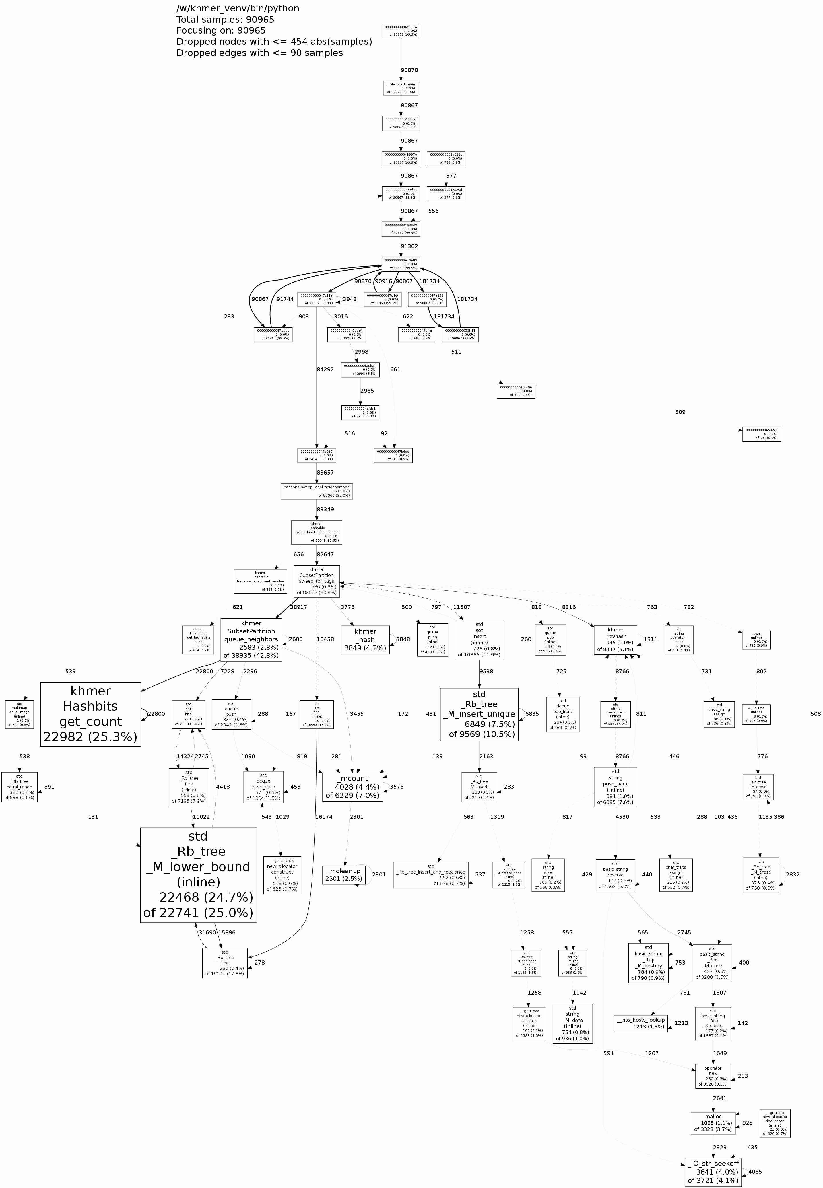
The resulting file is then visualized using google-pprof, with:

google-pprof --gif <python executable> <profile> > prof.gif

In order to get python debugging symbols, you need to use the debugging executable. So, while you may run the script in your virtualenv if using one, you give google-pprof the debug executable so it can properly construct callgraphs:

python -m yep -- /w/khmer/scripts/sweep-reads-by-partition-buffered.py \
 -k 25 -x 1e9 -o test_sweep -i /w/tests/test-sweep-contigs.fp \
/w/tests/test-sweep-reads.fa
google-pprof --gif /usr/bin/python2.7-dbg \
 sweep-reads-by-partition-buffer.py.prof > prof.gif

Results

Here is some example output:

In this call graph, the python debugging symbols were not properly included; this is resolved by using the debugging executable.

The call graph is in standard form, where the first percentage is the time in that particular function alone, and where the second percentage is the time in all functions called by that function. See the description for more details.

And that’s it. Happy profiling!